Nobody told it what a noun is
I trained a very small language model on four novels for five minutes. It had one task: predict the next word. I never mentioned grammar. At the end, nouns, verbs, adjectives and adverbs sat in different regions inside the model, and a simple test could read a word's class from its position 83 % of the time. Then I shuffled the words inside each sentence and trained again. This time, nothing of the kind happened.
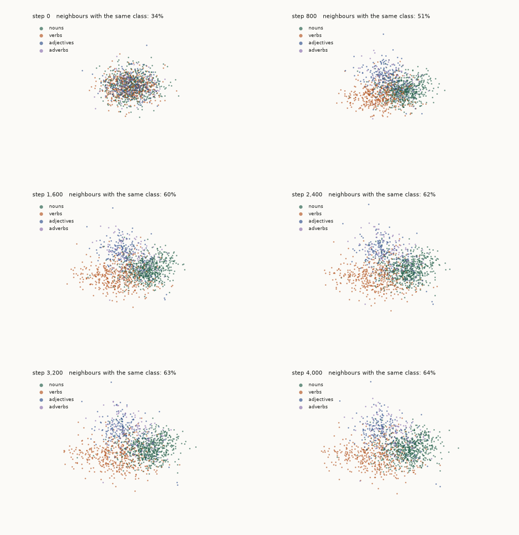
This post explains why that happens, why it is hard to show honestly, and what it tells you about the categories inside a language model.
The claim
You do not have to teach a language model word classes. They appear when the model learns to predict the next word. Words that occur in the same contexts receive the same corrections, so they move to the same place. “Noun” is the name that we give to one of the groups that form.
Hypothesis: why prediction alone gives word classes
If the claim is right, you can see it in a model small enough to inspect.
The model stores each word as a list of 64 numbers, called an embedding. Think of it as the position of the word in a space. Nobody tells the model that cat, river and hobbit belong together. But after training, their embeddings are near each other. The reason is in the training signal.
Take the word the. To predict what follows it, the model must find every word that can follow it: nouns and adjectives. The cheapest way is to make all those words look similar. Now take a noun. To predict what follows cat, river or hobbit, the model must find verbs such as was, ran and sat. The cheapest way is again to make the nouns similar to each other, and the verbs similar to each other. Each context that a class of words shares is one more push in the same direction.
So the model does not discover a label called “noun”. A noun is a member of an equivalence class under prediction: the set of words for which the same predictions are useful, about what comes before and about what comes after. Linguists call this a distributional definition, and it is older than neural networks. Training adds a way to find these classes in plain text, with nobody specifying them.
Three consequences:
- The class has degrees. Light is a noun and an adjective. It lands between the two groups, because its contexts are mixed.
- Word class is only one direction. The same pressure also groups words by tense, number, topic and mood, all at once, in different directions of the same space.
- A rare word does not move. A word that the model sees once receives one small correction and stays where it started. The effect needs repetition, so the size of the text decides whether you see anything.
Where the idea comes from: memory that you address by content
Attention uses three words: query, key and value. They come from an older idea in computer science. If you follow that idea, you see why attention has the shape it has.
Ordinary computer memory is addressed by location. array[5] gives you the contents of slot 5, and you must already know the slot. A content-addressable memory works the other way round. You show it a piece of content, and it gives you the entry that matches. In hardware this is a CAM chip, which compares the input with every stored word at the same time. Network routers and processor caches still use them. In software the same idea is a dictionary: sounds["cat"] looks up the key "cat" and gives back the value "meow". You never say where the entry is. The match finds it.
key: "cat"  → value: "meow"
key: "dog"  → value: "bark"

query: "cat"  → matches the key "cat"  → returns "meow"
This is the right kind of question for language. In “the cat sat because it was tired”, what does it refer to? You do not know that the answer is three positions back. You know what kind of thing you want, and you want the memory to find it.
Two differences separate a dictionary from attention. The history of the idea is the history of removing them.
The exact match became a soft match. A dictionary finds the key or it fails. A Hopfield network (1982) could already retrieve a stored pattern from a partial or noisy cue. The Neural Turing Machine (2014) gave the modern form: score the query against every memory slot, turn the scores into weights that sum to 1, and read out a weighted mix of all the slots. That is the attention formula. But the program still wrote the contents of the memory.
Stored entries became learned entries. In a dictionary, a person writes every key and value. Bahdanau, Cho and Bengio (2014) let a translation model use its own internal states as the memory, and the model learned how to score them. The Transformer (2017) took the last step. The query, the key and the value are each a learned view of the same embedding, so no person writes any part of the lookup. The paper named the three parts after the lookup that they generalise.
A note on who was first. Schmidhuber's fast weight programmers (1991) have one network write the weights of another, with vectors that act like keys and values, read out by a query. Schlag, Irie and Schmidhuber (2021) show that this is a linear form of the same idea, without the step that turns scores into weights. That step, and the framing that scaled, came in 2014 to 2017. This is why most people date attention to those years and he dates it to 1991.
The second difference is the hard one. A neural network has no entries stored in advance. Words arrive as vectors that start random. Nobody labels them, and nobody can say in advance what makes a good match. So the network must learn how to search and what to find at the same time, from a signal that mentions neither.
The solution has three parts:
- Learn three matrices,
W_Q,W_KandW_V, that turn an embedding into a query, a key and a value. - Measure similarity with the dot product. It is cheap enough to compute against every key, and smooth enough to learn from.
- Let one loss control all three, so that the same errors shape the search and the thing searched for.
| classical content-addressable memory | attention | |
|---|---|---|
| query | written by the program | W_Q e, learned |
| keys | written by the program | W_K e, learned |
| values | stored by the program | W_V e, learned |
| match rule | exact, or a fixed similarity | dot product, with a learned meaning |
| selection | best match | weighted mix of all matches |
| what the keys mean | designed | comes from the prediction loss |
The last row is the subject of the rest of this post.
Attention, in one page
Here is what one attention layer computes, and what the training signal sees. The first tells you where the classes can live. The second tells you why nothing else could have put them there.
Take “the cat sat because it was tired” and the word cat. The word has three jobs:
- As a key, cat must be easy to find for the searches that will look for it later: a pronoun that looks for the thing it refers to, a verb that looks for its subject. Its key carries something like “singular, alive, a noun that can act”.
- As a query, cat does its own search: for the article before it, and for anything that describes it. Its query must reach the and nearby adjectives, and ignore a verb three words away.
- As a value, cat decides what to hand over when it is selected. When it attends to cat, the useful content is “the subject is a small animal, singular”, not the spelling of the word.
The same word does all three jobs, and each job uses a different view of the same embedding:
q_i = W_Q e_i     query:  the search that this position sends to earlier positions
k_i = W_K e_i     key:    the label that this position shows, so that queries can match it
v_i = W_V e_i     value:  the content that is copied if this position is selected
Think of a job market. The query is the job advert. The key is the headline on a CV. The value is the work that the person does after they are hired. It is one person and three documents, and each document is written for one purpose.
The split between matching (Q and K) and content (V) is important. One vector does not have to be a good address and a good payload at the same time. Nobody writes these descriptions. The three matrices arrive at them because they make the next word easier to predict.
The three operations
For the word at position i, attention is three lines:
score_j  = q_i · k_j                       one score for each earlier position j
w_j      = exp(score_j) / Σ exp(score_m)   softmax: scores → weights that sum to 1
output_i = Σ w_j v_j a mix of the values, by weight- The dot product measures alignment. Two vectors that point the same way get a high score.
- The softmax turns the scores into weights. A few positions that match well get most of the weight, with no hard cut-off.
- The weighted sum lets several positions contribute. When it could refer to two things, the mix keeps both.
Now compute the output for it. Stage one scores the query of it against every key. Suppose that the weights are [0.02, 0.15, 0.05, 0.06, 0.14, 0.09, 0.49] for the, cat, sat, because, it, was, tired. These numbers are for illustration. In a trained model, cat would usually get the most weight for a pronoun.
Stop and look at what these numbers are: one share for each position. They say from whom to take, and nothing else. From this list alone, you cannot tell what cat is.
Stage two moves the content. Give each word a value of two numbers. The first means “animal” and the second means “state”: v_cat = [1, 0], v_tired = [0, 1], and every other word [0, 0]. Then:
output_it = 0.15·[1, 0] + 0.49·[0, 1] + 0.02·[0, 0] + … = [0.15, 0.49]This vector replaces the plain “I am the word it” at position 5. Position 5 now holds a little of cat and a lot of tired, so the output layer can prefer was to ran.
Attention is a gather. Each position rewrites itself as a weighted average of the values of all positions. Q·K answers “from whom?”. V answers “what?”. The sum is the act of taking it. Attention returns the value and not the key for the same reason that a dictionary does: the key is made to be found, and the value is made to be useful when found.
What the training optimises, and what it never sees
The loss is one number: how much probability the model gave to the word that came next. That is the complete training signal. Nothing checks the attention weights. Nothing tells the model that it should point at cat, or which words are nouns.
Many explanations, and my own first draft, say that training “compares the attention weights with the correct answer”. It does not. That difference is the point of this post.
For each example, the loop is:
- Forward: embed the words, run attention, and give a probability to every word in the vocabulary as the next word.
- Loss:
−log p(actual next word). - Backward: the error flows back through the output layer, the weighted sum, the softmax and the scores, into
W_Q,W_K,W_Vand the embeddings. - Step: each parameter moves a little in the direction that makes the right word more probable.
So q · k has no built-in meaning of “relevance”. If more weight on cat helps to predict was, the update turns q_it and k_cat towards each other. If weight on because hurts, it turns them apart. After millions of these small updates, the dot product encodes what is useful to attend to, because that is the only way to lower the loss. Nobody defines relevance. It is what remains after optimisation.
“Turn” is the correct word. The score is q · k = |q| |k| cos θ, so a high score and a small angle are the same fact. And the derivative of q_it · k_cat with respect to q_it is k_cat. When the loss asks for a higher score on cat, the update adds a little of k_cat to q_it, and a little of q_it to k_cat. That is a rotation towards each other. “Make this score larger” and “align these two vectors” are one operation.
There is no deep reason why the dot product must work. It works because it is cheap, smooth and flexible enough for training to shape the matrices into a solution.
Three ways to cheat
This is harder to show in a small demo than it sounds. Each shortcut that makes the picture clean also makes it meaningless. I tried three before the run below. You have probably seen all three in other explanations.
| attempt | what it did | why it does not count |
|---|---|---|
| k-means on the embeddings | grouped the points with a clustering algorithm | we added the groups, the model did not learn them; the algorithm finds groups in noise too |
| designed sentences | 8 words, each noun followed by it, each verb by a verb | the classes were built into the data; the model could only repeat them |
| 60 hand-written sentences | natural text, but about 140 words, each seen once or twice | too little repetition: the loss fell, the embeddings almost did not move |
Setup
The run that counts uses none of these:
- Text: four published novels, not edited: Jane Austen's Emma, Persuasion and Sense and Sensibility, and Lewis Carroll's Alice's Adventures in Wonderland. Together they have about 394,000 words. The vocabulary is the 3,110 words that occur 8 times or more.
- Model: one attention head over embeddings of 64 numbers, with a residual connection and an output layer. It has about 420,000 parameters. It is trained on the next-word loss only.
- Labels: a separate program, the NLTK part-of-speech tagger, gives each word a class afterwards. The model never sees these labels.
- Measured words: the 1,320 nouns, verbs, adjectives and adverbs that occur 25 times or more.
Two numbers show whether word classes have appeared:
- Neighbours. For each word, take its 10 nearest words in the embedding space. What share of them has the same class?
- Probe. Train a simple linear classifier to read the class of a word from its embedding. How often is it right on words that it did not train on?
Each number has a chance level. For the neighbours, it is the share you get if the words are placed at random. For the probe, it is the score you get if you always answer “noun”.
Results
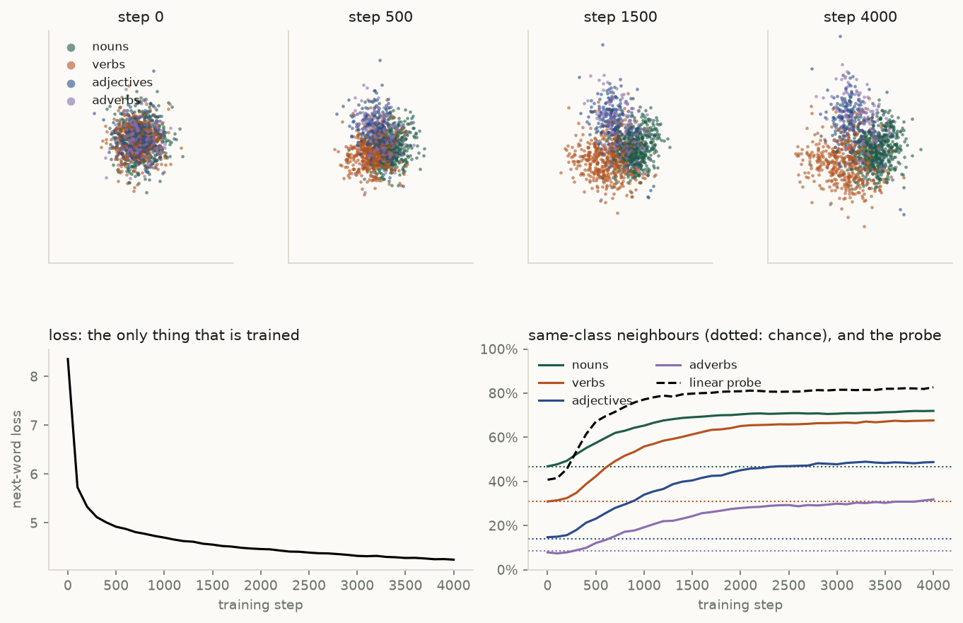
Training took 4,000 steps, about five minutes on a laptop.
| measure | before training | after 4,000 steps | chance |
|---|---|---|---|
| neighbours with the same class, all words | 34 % | 64 % | 34 % |
| nouns | 47 % | 72 % | 47 % |
| verbs | 31 % | 68 % | 31 % |
| adjectives | 15 % | 49 % | 14 % |
| adverbs | 8 % | 32 % | 8 % |
| probe reads the class from the embedding | 41 % | 83 % | 47 % |
Before training, every number is at chance. There is no structure at the start. After five minutes, the neighbours of a word share its class almost twice as often as chance, and the probe reads the class correctly 83 % of the time. The loss went from 8.4 to 4.25 in the same steps. The loss falls and the two measures rise together.
The control: the same words, with the order destroyed
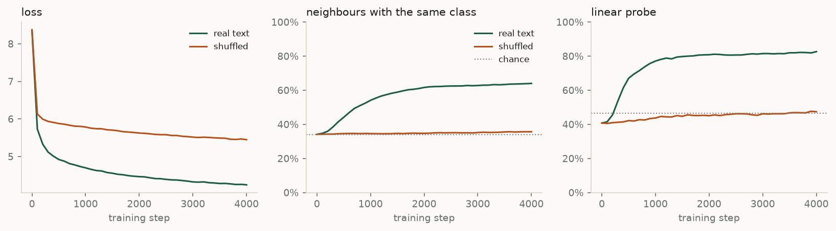
You can still doubt this result. The structure could come from something other than word order: from how frequent a word is, from which words share a sentence, or from the tagger. So I ran the same model on the same text with one change. I shuffled the words inside each sentence. Each word keeps its frequency and the other words of its sentence. Only the order is gone.
| measure | real text | shuffled | chance |
|---|---|---|---|
| loss after 4,000 steps | 4.25 | 5.45 | 8.04 at the start |
| neighbours with the same class | 64 % | 36 % | 34 % |
| nouns / verbs / adjectives / adverbs | 72 / 68 / 49 / 32 | 49 / 32 / 15 / 9 | 47 / 31 / 14 / 8 |
| probe reads the class | 83 % | 47 % | 47 % |
The shuffled model still learns. Its loss falls from 8.4 to 5.45, because it can still learn which words are frequent and which words occur in the same sentence. But both measures stay at chance. Word classes come from what stands next to a word, and the shuffle removes exactly that.
Why this matters
The point is not nouns. A category that nobody specified appeared as a side effect of a task that never mentioned it, in a model small enough to read.
The same mechanism runs in a production language model, with thousands of these directions and not four: tense, number, mood, style, topic, and things that have no name. Each one is a direction that made prediction cheaper.
When people argue about whether a language model “understands” grammar, this is the concrete thing they are arguing about. The model was not given a rule. The statistics of the text pushed it into a structure, and a linear probe can read that structure back.
Limitations
- The picture understates the result. The two axes of the scatter plots hold about 7 % of the variation in the 64 dimensions. The neighbours and the probe are measured in the full space. They are the evidence. The plot is an illustration. Other projection methods draw tighter groups, but they exaggerate groups by design, so I did not use them.
- The model is very small. It has one head and one layer, and it trains for minutes. It shows the mechanism, not the scale.
- The labels are not perfect. Each word gets the class that the tagger gave it most often. Part of the remaining 36 % is words that belong to two classes, such as light, back and close. Part is errors of the tagger. Part is structure along directions other than word class.
- “Noun” means the distributional class here, not a linguist's definition. In English the two agree most of the time, which is why the tagger and the model agree as much as they do.
- These are not the numbers of my first run. An earlier version of this post reported 67 % and 88 %, from a run whose code I did not keep. I wrote the experiment again from its description, and all numbers and figures here come from that code, which is public.
Run it yourself
The quickest way is the notebook. Open it in Colab and it runs in your browser, with nothing to install. It shows the text and the labels, trains the model in a short run of about a minute, draws the figures from the saved runs, and lets you look up the nearest neighbours of any word.
To run the full experiment on your own machine, you need PyTorch and NLTK. It runs on a CPU and takes about five minutes for each run.
pip install torch nltk numpy matplotlib
python attn_emergence.py 4000            # the real run
python attn_emergence.py 4000 --shuffle  # the control
python viz_emergence.py                  # the figures and the table
The code is here: attn_emergence.py and viz_emergence.py, with the saved results of both runs. The first run downloads the novels and the tagger.
Two things to try. Change the text: any text of the NLTK Gutenberg collection works, and Moby Dick is a good one. Or change the size of the embeddings: 32 numbers still work, and 8 almost do not.
Sources
- Texts: Emma, Persuasion and Sense and Sensibility (Jane Austen) and Alice's Adventures in Wonderland (Lewis Carroll), from Project Gutenberg as packaged in the NLTK Gutenberg corpus.
- Part-of-speech labels: the NLTK averaged-perceptron tagger with the universal tagset. Each word gets its most frequent label.
- The history: Hopfield, “Neural networks and physical systems with emergent collective computational abilities” (1982); Graves, Wayne and Danihelka, “Neural Turing Machines” (2014); Bahdanau, Cho and Bengio, “Neural Machine Translation by Jointly Learning to Align and Translate” (2014); Vaswani et al., “Attention Is All You Need” (2017).
- The distributional view of word classes: Harris, “Distributional Structure” (1954).